So there has been quite a bit of talk on Big Data processing, High Performance Computing (HPC), clusters (grouping of computers), supercomputing and such. Our world has gone digital and with that we have more data than we know what to do with and to process this data in a timely fashion we need systems with more power. Ultimately, as processing needs increase so does the world of supercomputing.
So where did the madness begin?
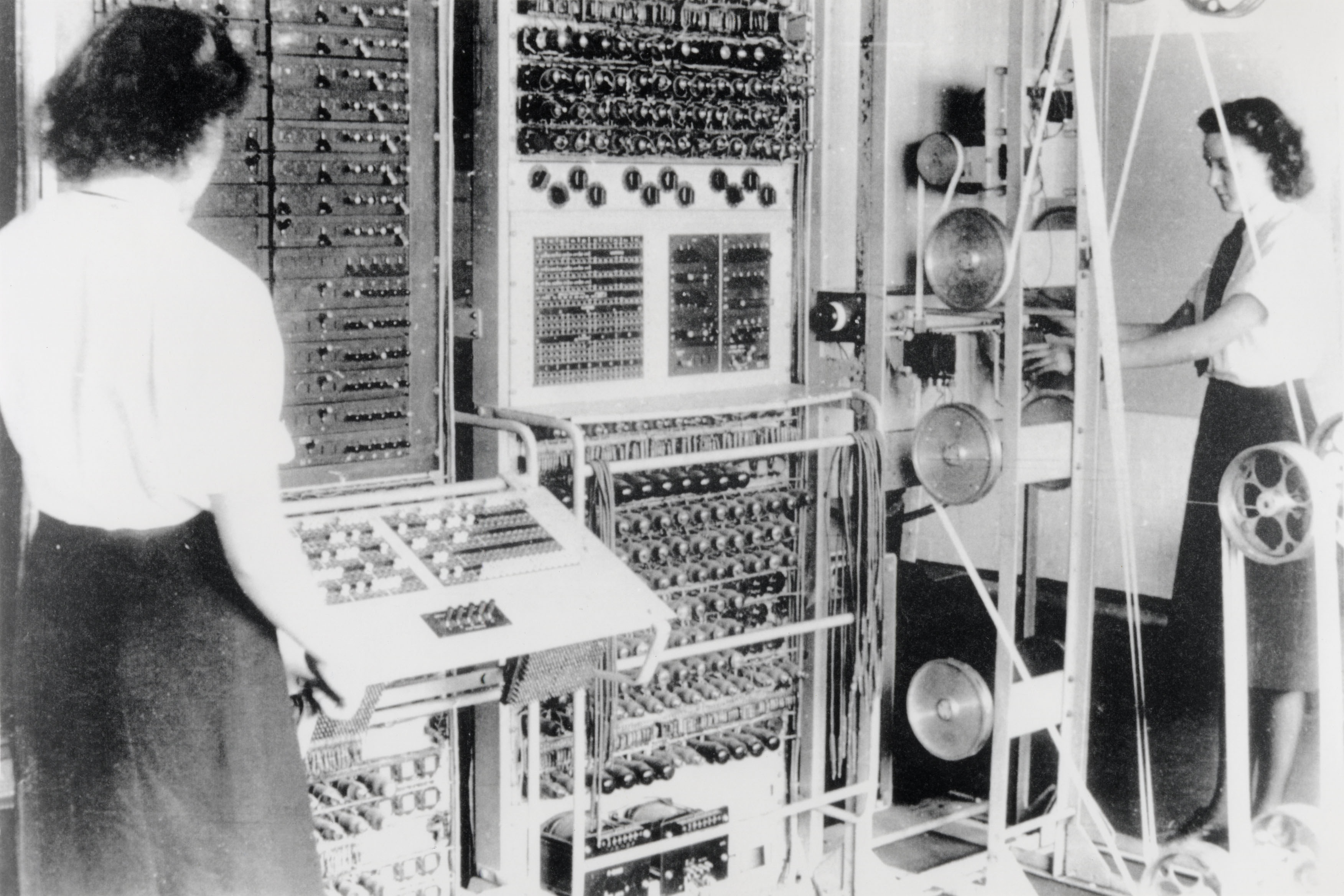
One of the first supercomputers was the Colossus! Built in 1943, this vacuum tube device was the first digital, programmable computer. It was used to crack the Enigma code used by Germans during World War II. Totally awesome, this device helped the Allied Forces decipher German telegraphic messages and seriously aided in providing military intelligence.
In 1944,the Harvard Mark I was completed. It was the first large-scale general purpose computer. The Mark I computer was tested as the first computer to be able to store data along with programs. Its successor known as the Mark II was built in 1945. One day a moth was found caught within the computer, the moth was removed resulting in the first debugging of a computer.
In 1946, the Electronic Delay Storage Automatic Calculator (ENIAC) was assembled by the Moore School at the University of Pennsylvania, it came down for a short period of time but was continuously powered on in 1947. It consisted of 19,000 vacuum tubes and was used by the government to test the feasibility of the hydrogen bomb along with other War World II ballistic firing tables.
One of the first UK computers, Pilot Ace ran at one million cycles per second in 1950. Following, the UNIVAC processed election data and accurately predicted the winner of the 1952 presidential elections. The computer said Eisenhower would win by a landslide despite polls predicting Adlai Stevenson. General Electric used this computer system to process their payroll paying $1 million for the services. The more versatile stored computer, EDVAC was built in the US around 1951. It differed from UNIVAC by using binary over decimal numbers and only consisted of 3,500 tubes.

Continuing, IBM contributes to supercomputing with their 701 (Defense Calculator). It was used for scientific calculations and provided a transition from punch cards to electronic computers in 1952. That same year, the MANIAC I was built. It was also used for scientific computations and helped in the engineering of the hydrogen bomb.
In 1953, the first real-time video was displayed on MIT’s Whirlwind computer.

IBM made great strides in supercomputing, they introduced the rugged 650 in 1954 and the 704, the first computer to fully deploy floating-point math in 1955. IBM’s RAMAC, in 1956, was the first computer to use a hard disk while calculating high-volume business transactions. Following, their 7090 was a commercial scientific computer used for space exploration. In 1961, IBM develops the fastest supercomputer yet, the STRETCH. This was IBM’s first transistor computer. The transistors replaced the traditional vacuum tubes used at the time.
In 1962, the University of Manchester in the UK introduced Atlas, it was capable of using virtual memory, lagging and job scheduling. “It was said that whenever Atlas went offline half of the United Kingdom’s computer capacity was lost” (Wikipedia).

Semi-Automatic Ground Environment (SAGE) was completed in 1963. It connected 554 computers together and was used to detect air attacks. B5000, developed by Burroughs utilized high-level programming languages ALGOL and COBOL in multiprocessing operations. 1964, Control Data Corporation built the CDC 6600 maxing at 9 Megaflops. It was one of Seymour Cray (Yes, the same Cray from the Cray clusters) first designs.
IBM introduces System 360 in 1969. It is the first computer to include data and instruction cache memory. This line of computers stretched from performing scientific computations to commercial applications providing a broad use of capabilities.
In the 1970s, supercomputers became a source of national pride for producing countries. More than ever, computers were being commercialized with secular processors. This designed produced more of an all-in-one solution for most applications but typically lent to slower speeds.
In 1975, DEC KL-10, the first minicomputer that could compete in the mainframe market was produced by Digital. Minicomputers were a cheaper solution to other computer implementations.The New York Times, defined a minicomputer as a machine capable of processing high level programming languages, costing less than $25,000, with an input-output device and at least 4K words of memory.
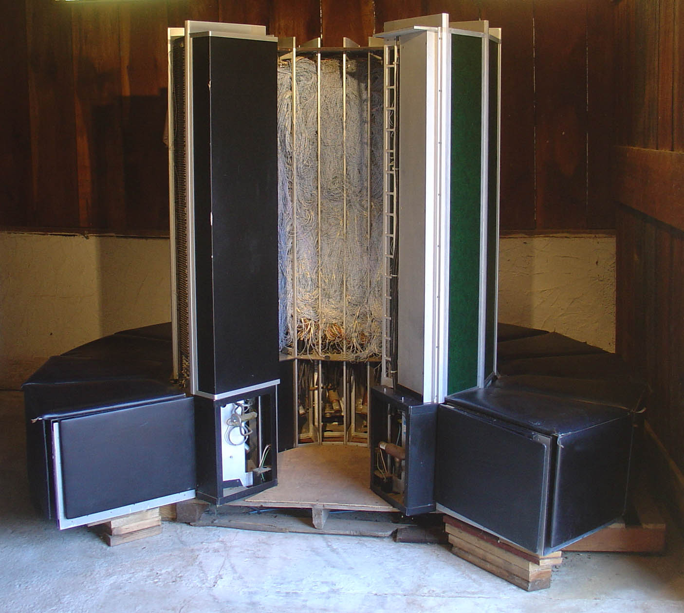
Seymour Cray, released the Freon-cooled Cray-1 in 1976. Freon is a cooling agent used in most air conditioning systems. This technology was used to keep cluster systems from overheating or reaching dangerous heat levels for maintenance workers. Cray was a flashy man, notice the cushion like structure around the Cray. People could now sit and enjoy their supercomputer.
In 1982, Fujitsu produced the VP-200 vector supercomputer. This new computer was able to process data at a rate of 500 Mflops.
The Cray-2 was released to the National Energy Research Scientific Computing Center in 1983 and consisted of eight processors. It was the fastest machine in the world at the time with four vector processors. Vector processing allowed an entire vector or array of data to be processed at a time. This significantly increased performance over secular methods.
More history to come in part two…