A History of Supercomputing because… I Feel Like It – Part Two

Now this isn’t an extensive history, right now I’m just posting major develops. At a later time, I might revise and beef up these posts because it really is cool to see how we have progressed from vacuum tubes to our modern beasts! Onward!

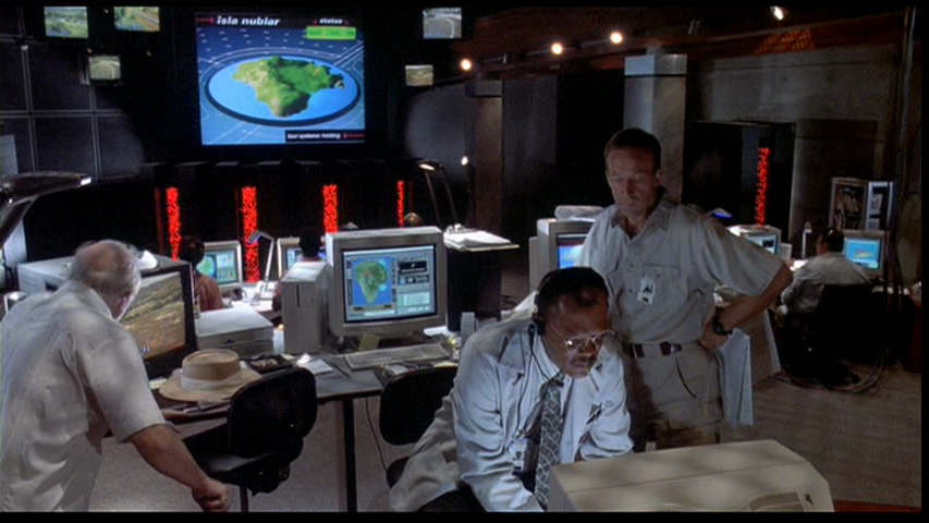
The next design for supercomputers involved individual processors each with their own 4kbit RAM memory (so cute compared to our GB memory now). This was earliest seen in 1985 with Thinking Machine’s Connection Machine 1. This design was an improvement over vector processing and provided a massively parallel infrastructure. Fun fact, the Connection Machine 5 had a vital role in Jurassic Park. It was the supercomputer in the control room!

Notice the red lights in the background.

Cost of vector computers continued to decrease as minicomputers improved their uniprocessor design with the Convex C1.

In 1988, NASA adopted the Cray Y-MP.  This new supercomputer could be equipped with 2,4, or 8 vector processors. It peaked at 333 Mflops per processor. Flops standing for floating-point operations per second.

1990, Intel introduced the Touchstone Delta Supercomputer. This device used 512 reduced instruction set computing (RISC) processors. RISC consists of simplified instructions over complex that are believed to increase performance because of the faster execution times.

Their was a brief lull in development around the end of cold war. This slowed down supercomputing progress.

In 1992, Intel continues their Delta line and builds the first Paragon supercomputer. This device consists of distributed memory multiprocessor systems with 32-bit RISC. Also that year, Cray ‘s C90 series reached a performance of one Gflop a big boost in performance.

In 1993, IBM promotes their SP 1 Power Parallel System. This device was based off of the Performance Optimization With Enhanced RISC – Performance Computing (PowerPC) infrastructure. PowerPC later evolved into Power ISA. This architecture was developed by the Apple-IBM-Motorola alliance and has been replaced by Intel in many personal computers but is still popular among embedded systems.

Cray Computer Corporation (founded in 1972) constructs their T3D. This was the corporation’s first attempt at a massively parallel machine. It was capable of scaling from 32 on up to 2,048 processors.

In 1994, the Beowulf Project came into play with their 16 node Linux cluster.  NASA used it for their Space Sciences project. The Beowulf Project has since evolved into the Beowulf cluster which consists of a local network of shared devices. Cool thing is that this project has helped to bring high performance computing power to connected personal devices.

Intel’s Accelerated Strategic Computing Initiative (ASCI) Red improved performance in 1997 on the LINPACK Benchmark at Sandia National Labs, reaching 1.3 Tflops. ASCI Blue continued to boost performance on  supercomputers, peaking at 3 Tflops in 1998 and ASCI White enabled 7.22 Tflops in 2000.

In 2002, the NEC uses supercomputing to run earth simulations at Japan’s Yokohama Institute for Earth Science. Think of how much data that involves! That same year, Linux clusters become popular, reaching 11 Tflops! I use Linux!

China’s Tianhe-1A,  located at the National Supercomputing Center in Tianjin, reaches 2.57Pflops, a huge, huge jump in performance. This became the world’s fastest computer in 2010. This reign was short lived and only lasted till Japan’s K computer by Fujitsu reached 8 Pflops in June of 2011 and 10 Pflops later that November. However, it is still one of the few petascale supercomputers in the world.

Supercomputing is still improving. In January 2012, Intel purchased the InfiniBand product line in hopes of meeting their promise of developing exascale technology by 2018. Wow! Again, more power results in an increase in data processing capabilities. Think of what else we could simulate with this type of technology, how much more detail will we be able examine?

Things are looking up.

A History of Supercomputing because… I Feel Like It – Part One

So there has been quite a bit of talk on Big Data processing, High Performance Computing (HPC), clusters (grouping of computers), supercomputing and such. Our world has gone digital and with that we have more data than we know what to do with and to process this data in a timely fashion we need systems with more power. Ultimately, as processing needs increase so does the world of supercomputing.

So where did the madness begin?

One of the first supercomputers was the Colossus! Built in 1943, this vacuum tube device was the first digital, programmable computer. It was used to crack the Enigma code used by Germans during World War II. Totally awesome, this device helped the Allied Forces decipher German telegraphic messages and seriously aided in providing military intelligence.

In 1944,the Harvard Mark I was completed. It was the first large-scale general purpose computer. The Mark I computer was tested as the first computer to be able to store data along with programs. Its successor known as the Mark II was built in 1945. One day a moth was found caught within the computer, the moth was removed resulting in the first debugging of a computer.

In 1946, the Electronic Delay Storage Automatic Calculator (ENIAC) was assembled by the Moore School at the University of Pennsylvania, it came down for a short period of time but was continuously powered on in 1947. It consisted of 19,000 vacuum tubes and was used by the government to test the feasibility of the hydrogen bomb along with other War World II ballistic firing tables.

One of the first UK computers, Pilot Ace ran at one million cycles per second in 1950.  Following, the UNIVAC processed election data and accurately predicted the winner of the 1952 presidential elections. The computer said Eisenhower would win by a landslide despite polls predicting Adlai Stevenson. General Electric used this computer system to process their payroll paying $1 million for the services. The more versatile stored computer, EDVAC was built in the US around 1951. It differed from UNIVAC by using binary over decimal numbers and only consisted of 3,500 tubes.

Continuing, IBM contributes to supercomputing with their 701 (Defense Calculator). It was used for scientific calculations and provided a transition from punch cards to electronic computers in 1952. That same year, the MANIAC I was built. It was also used for scientific computations and helped in the engineering of the hydrogen bomb.

In 1953, the first real-time video was displayed on MIT’s Whirlwind computer.

IBM made great strides in supercomputing, they introduced the rugged 650 in 1954 and the 704, the first computer to fully deploy floating-point math in 1955. IBM’s RAMAC, in 1956, was the first computer to use a hard disk while calculating high-volume business transactions. Following, their 7090 was a commercial scientific computer used for space exploration. In 1961, IBM develops the fastest supercomputer yet, the STRETCH. This was IBM’s first transistor computer. The transistors replaced the traditional vacuum tubes used at the time.

In 1962, the University of Manchester in the UK introduced Atlas, it was capable of using virtual memory, lagging and job scheduling. “It was said that whenever Atlas went offline half of the United Kingdom’s computer capacity was lost” (Wikipedia).

Semi-Automatic Ground Environment (SAGE) was completed in 1963. It connected 554 computers together and was used to detect air attacks. B5000, developed by Burroughs utilized high-level programming languages ALGOL and COBOL in multiprocessing operations.  1964, Control Data Corporation built the CDC 6600 maxing at 9 Megaflops. It was one of Seymour Cray (Yes, the same Cray from the Cray clusters) first designs.

IBM introduces System 360 in 1969. It is the first computer to include data and instruction cache memory. This line of computers stretched from performing scientific computations to commercial applications providing a broad use of capabilities.

In the 1970s, supercomputers became a source of national pride for producing countries. More than ever, computers were being commercialized with secular processors. This designed produced more of an all-in-one solution for most applications but typically lent to slower speeds.

In 1975, DEC KL-10, the first minicomputer that could compete in the mainframe market was produced by Digital. Minicomputers were a cheaper solution to other computer implementations.The New York Times, defined a minicomputer as a machine capable of processing high level programming languages, costing less than $25,000, with an input-output device and at least 4K words of memory.

Seymour Cray, released the Freon-cooled Cray-1 in 1976. Freon is a cooling agent used in most air conditioning systems. This technology was used to keep cluster systems from overheating or reaching dangerous heat levels for maintenance workers. Cray was a flashy man, notice the cushion like structure around the Cray. People could now sit and enjoy their supercomputer.

In 1982,  Fujitsu produced the VP-200 vector supercomputer. This new computer was able to process data at a rate of 500 Mflops.

The Cray-2 was released to the National Energy Research Scientific Computing Center in 1983 and consisted of eight processors. It was the fastest machine in the world at the time with four vector processors. Vector processing allowed an entire vector or array of data to be processed at a time. This significantly increased performance over secular methods.

More history to come in part two…